

16.1 Properties Of Logarithms Answers
This volume is in Open Review. We want your feedback to make the book better for yous and other students. You may comment some text by selecting it with the cursor and then click the on the popular-up menu. You can as well see the annotations of others: click the in the upper correct hand corner of the page
Regression when X is a Binary Variable
Instead of using a continuous regressor \(X\), we might be interested in running the regression
\[ Y_i = \beta_0 + \beta_1 D_i + u_i \tag{5.2} \]
where \(D_i\) is a binary variable, a and so-called dummy variable. For example, we may define \(D_i\) as follows:
\[ D_i = \begin{cases} i \ \ \text{if $STR$ in $i^{th}$ school district < twenty} \\ 0 \ \ \text{if $STR$ in $i^{th}$ school district $\geq$ xx} \\ \end{cases} \tag{5.3} \]
The regression model at present is
\[ TestScore_i = \beta_0 + \beta_1 D_i + u_i. \tag{5.4} \]
Let united states see how these data look like in a scatter plot:
# Create the dummy variable as defined in a higher place CASchools$D <- CASchools$STR < xx # Plot the data plot(CASchools$D, CASchools$score, # provide the data to exist plotted pch = 20, # use filled circles equally plot symbols cex = 0.five, # set size of plot symbols to 0.5 col = "Steelblue", # set the symbols' color to "Steelblue" xlab = expression(D[i]), # Ready title and axis names ylab = "Exam Score", main = "Dummy Regression") 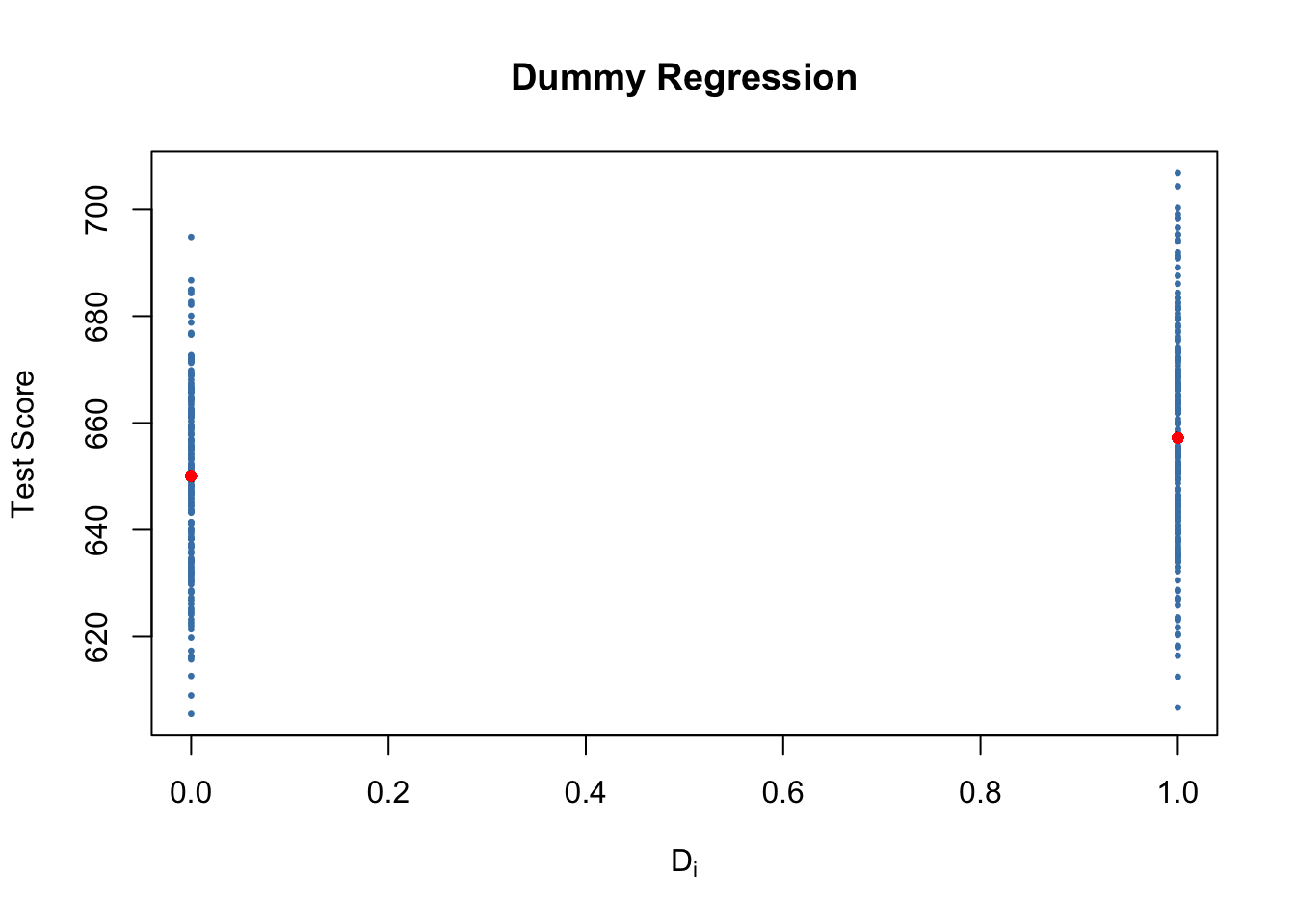
With \(D\) as the regressor, it is not useful to recall of \(\beta_1\) as a slope parameter since \(D_i \in \{0,ane\}\), i.e., we only observe two discrete values instead of a continuum of regressor values. There is no continuous line depicting the conditional expectation function \(E(TestScore_i | D_i)\) since this role is solely defined for \(x\)-positions \(0\) and \(1\).
Therefore, the interpretation of the coefficients in this regression model is equally follows:
-
\(East(Y_i | D_i = 0) = \beta_0\), and so \(\beta_0\) is the expected test score in districts where \(D_i=0\) where \(STR\) is higher up \(20\).
-
\(E(Y_i | D_i = i) = \beta_0 + \beta_1\) or, using the result above, \(\beta_1 = Due east(Y_i | D_i = i) - East(Y_i | D_i = 0)\). Thus, \(\beta_1\) is the difference in group-specific expectations, i.due east., the difference in expected exam score between districts with \(STR < xx\) and those with \(STR \geq xx\).
We will at present apply R to estimate the dummy regression model equally defined by the equations (5.2) and (v.3) .
# estimate the dummy regression model dummy_model <- lm(score ~ D, information = CASchools) summary(dummy_model) #> #> Telephone call: #> lm(formula = score ~ D, data = CASchools) #> #> Residuals: #> Min 1Q Median 3Q Max #> -fifty.496 -xiv.029 -0.346 12.884 49.504 #> #> Coefficients: #> Estimate Std. Error t value Pr(>|t|) #> (Intercept) 650.077 1.393 466.666 < 2e-16 *** #> DTRUE vii.169 i.847 3.882 0.00012 *** #> --- #> Signif. codes: 0 '***' 0.001 '**' 0.01 '*' 0.05 '.' 0.1 ' ' one #> #> Residual standard error: eighteen.74 on 418 degrees of freedom #> Multiple R-squared: 0.0348, Adjusted R-squared: 0.0325 #> F-statistic: xv.07 on 1 and 418 DF, p-value: 0.0001202 reports the \(p\)-value of the test that the coefficient on
(Intercept)is zero to to be
< 2e-16. This scientific notation states that the \(p\)-value is smaller than \(\frac{2}{10^{16}}\), then a very small number. The reason for this is that computers cannot handle capricious small numbers. In fact, \(\frac{2}{10^{16}}\) is the smallest possble number
Rcan work with.
The vector CASchools$D has the type logical (to encounter this, use typeof(CASchools$D)) which is shown in the output of summary(dummy_model): the label DTRUE states that all entries TRUE are coded as one and all entries FALSE are coded every bit 0. Thus, the interpretation of the coefficient DTRUE is equally stated above for \(\beta_1\).
One can run across that the expected test score in districts with \(STR < xx\) (\(D_i = 1\)) is predicted to be \(650.i + 7.17 = 657.27\) while districts with \(STR \geq 20\) (\(D_i = 0\)) are expected to accept an average test score of only \(650.one\).
Group specific predictions can be added to the plot by execution of the post-obit code chunk.
# add grouping specific predictions to the plot points(10 = CASchools$D, y = predict(dummy_model), col = "red", pch = 20) Here we use the function predict() to obtain estimates of the grouping specific means. The blood-red dots represent these sample group averages. Accordingly, \(\hat{\beta}_1 = 7.17\) can exist seen as the difference in group averages.
summary(dummy_model) also answers the question whether at that place is a statistically significant departure in group ways. This in turn would support the hypothesis that students perform differently when they are taught in small classes. We can appraise this by a 2-tailed test of the hypothesis \(H_0: \beta_1 = 0\). Conveniently, the \(t\)-statistic and the corresponding \(p\)-value for this test are computed past summary().
Since t value \(= 3.88 > 1.96\) we reject the null hypothesis at the \(5\%\) level of significance. The same decision results when using the \(p\)-value, which reports significance upwardly to the \(0.00012\%\) level.
As done with linear_model, nosotros may alternatively use the function confint() to compute a \(95\%\) confidence interval for the truthful deviation in means and see if the hypothesized value is an element of this conviction set.
# confidence intervals for coefficients in the dummy regression model confint(dummy_model) #> 2.5 % 97.v % #> (Intercept) 647.338594 652.81500 #> DTRUE 3.539562 ten.79931 We reject the hypothesis that at that place is no difference between group means at the \(v\%\) significance level since \(\beta_{1,0} = 0\) lies outside of \([three.54, 10.8]\), the \(95\%\) confidence interval for the coefficient on \(D\).

16.1 Properties Of Logarithms Answers,
Source: https://www.econometrics-with-r.org/5-3-rwxiabv.html
Posted by: kotterscurinter.blogspot.com
0 Response to "16.1 Properties Of Logarithms Answers"
Post a Comment